Can PCB Simulation Prevent Costly Manufacturing Revisions?
14 min
- What Is PCB Simulation and Why Does It Matter?
- Four PCB Simulation Areas That Affect Board Performance
- Turn Simulation Results into a Manufacturing-Ready PCB
- How JLCPCB Capabilities Support Simulation-Driven Designs
- FAQs about PCB Simulation
- Conclusion
Key Takeaways
- PCB simulation identifies electrical, thermal, and EMC issues before fabrication, helping reduce costly design revisions.
- Signal integrity, power integrity, thermal, and EMC analysis address different PCB performance risks.
- Accurate simulation depends on matching the model to the actual stackup, materials, and manufacturing limits.
- Combining simulation with DRC checks and prototype testing helps ensure reliable, manufacturable PCB designs.
PCB simulation is the practice of predicting how a board will behave, electrically and thermally, from its schematic, stackup, and layout before any copper is etched. It covers circuit behavior, signal and power integrity, heat, and electromagnetic emissions. Each of these failure classes otherwise appears only on a prototype. Each one found there costs a new layout, a new fabrication lead time, and a new assembly run.
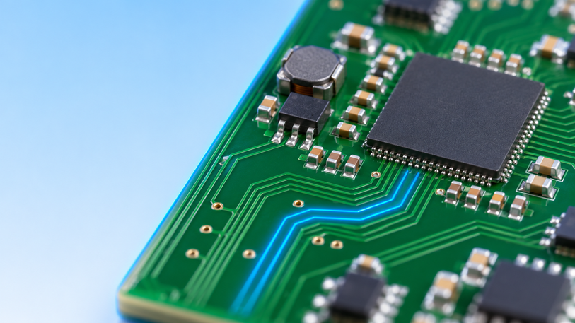
Figure 1: A multilayer board where simulation predicts heat, noise, and signal behavior
This article explains what simulation can and cannot capture, as well as the four areas of analysis that affect board performance. It then shows how to carry the results into a stackup, design rules, and fabrication data that the manufacturer builds as modeled.
What Is PCB Simulation and Why Does It Matter?
PCB simulation is part of the build-and-measure iteration loop and is being replaced by calculation. It's important because most board modifications are due to effects not shown on the schematic: trace impedance, plane resistance, heat flow, and current return paths, all of which are geometry-related.
Circuit Simulation vs. PCB-Level Simulation
Circuit simulation performs the following operations: Solving the schematic. A SPICE engine assumes all nets in the circuit to be ideal (no length, no resistance, no coupling to others). Then it performs DC, AC, and transient voltage/ current calculations. That's the correct level of abstraction for looking at a filter's corner frequency, regulator loop stability, etc. At those frequencies and currents, the wiring is really not important, and the ideal nets give the correct answer.
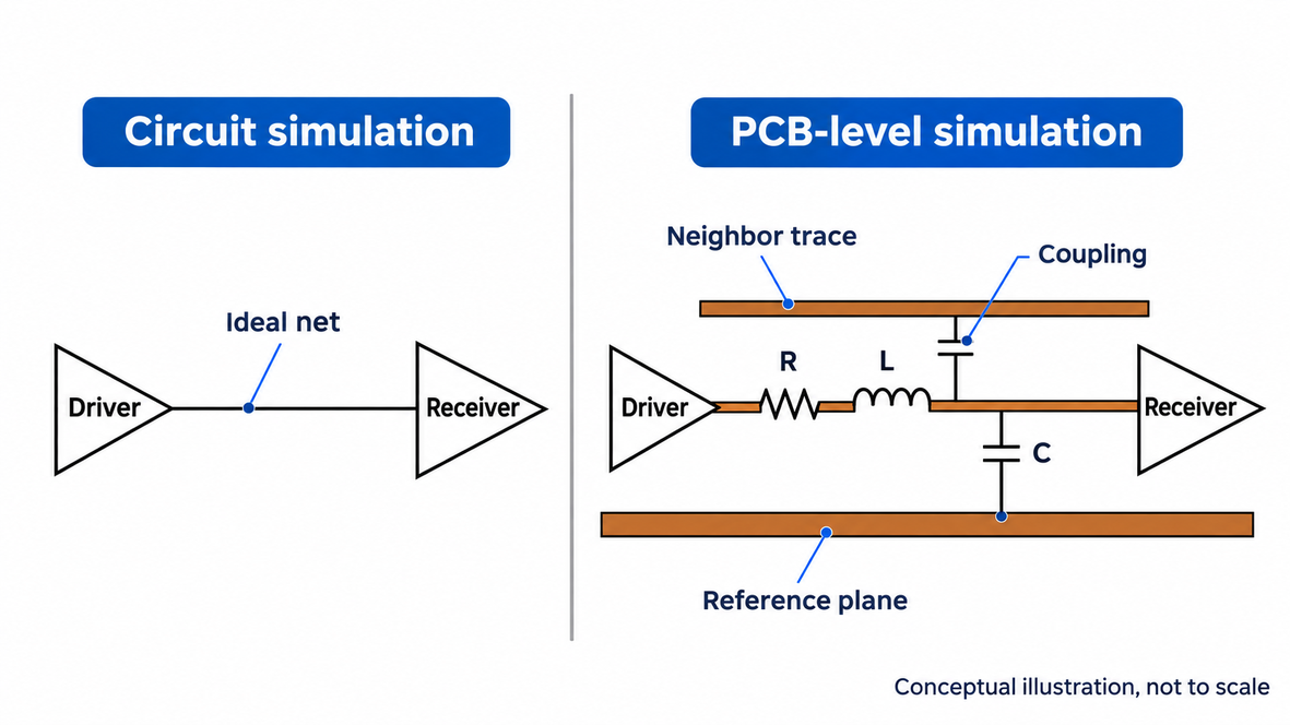
Figure 2: An ideal schematic net vs. the same net with layout parasitics
The layout is solved using PCB-level simulation. The trace geometry, the stackup, and the reference planes are read by a field solver. It then removes the resistance, inductance, capacitance, and coupling introduced by the copper. It is those parasitics that make a good schematic a board that rings, droops, or radiates. Circuit simulation can tell you if the design will work in principle, and PCB-level simulation can tell you if this particular layout will work.
How Simulation Supports PCB Design and Manufacturing
Each analysis belongs at the point where its inputs first exist. Circuit simulation runs on the schematic, before layout. Stackup and impedance calculations run before routing, because the trace widths depend on them. Signal integrity checks run on critical nets during routing. Once the layout is finished, the full post-layout set of signal integrity, power integrity, thermal, and EMC checks runs on the real geometry before the design is released.
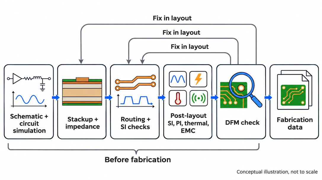
Figure 3: Where each simulation step sits in the PCB design flow
So, can simulation prevent costly revisions? For problems that follow from geometry and known models, largely yes. An impedance mismatch, an undersized power plane, a hot regulator, or a crosstalk-prone pair can all be found and fixed in the layout. However, simulation cannot catch a wrong footprint, a pin swap in a symbol, or an assembly defect. Its answers are also only as good as its inputs, so a model built on a stackup the fabricator does not use predicts a board that will never exist.
Four PCB Simulation Areas That Affect Board Performance
The four areas are circuit simulation, signal and power integrity, thermal and multiphysics analysis, and electromagnetic compatibility. They differ in what they model, what they need as input, and which failure they prevent.
| Simulation Area | What It Models | Typical Inputs | Failure It Prevents |
|---|---|---|---|
| Circuit simulation | Component behavior on ideal nets | Schematic, SPICE models | Wrong gain, unstable loops, bad startup |
| Signal and power integrity | Waveforms and supply noise on real copper | Layout, stackup, IBIS and capacitor models | Ringing, crosstalk, timing errors, supply droop |
| Thermal and multiphysics | Heat flow and temperature rise | Power dissipation, copper, vias, airflow | Hot spots, derated parts, joint stress |
| Electromagnetic compatibility | Emissions and susceptibility | Layout, planes, cables, enclosure | Failed emissions tests, interference |
Circuit Simulation for Functional Validation
Before anyone takes a trace, circuit simulation verifies that the circuit does what the schematic says. A DC operating-point analysis verifies bias points and ensures all regulators' outputs/references are where they should be. AC analysis yields the filter responses and amplifier bandwidth; transient analysis displays the startup behavior, switching waveforms, and the control loop's response to a load step.
The outcome depends on models and on part dispersion. Where they exist, use the manufacturer's model for op-amps, regulators, and MOSFETs, as it will capture device behavior not included in the generic model, e.g., output voltage swing limits for op-amps or gate charge for MOSFETs. Next, a parameter sweep is performed over the component tolerances and temperature, revealing that the design is viable only if all parts are at their nominal values. This condition would be discovered on the production line.
Signal and Power Integrity for High-Speed PCBs
Signal integrity simulation enables prediction of the appearance of a digital edge at the receiver. A trace electrically becomes a transmission line when it is longer than the rise time of the edge. Any impedance discontinuity along it, however, whether via, stub, or lack of termination, reflects part of the signal back to the driver. The simulator models the driver's IBIS and a behavioral model of the I/O buffer to simulate the line. It displays overshoot, ringing, crosstalk, and plots eye diagrams for serial links.
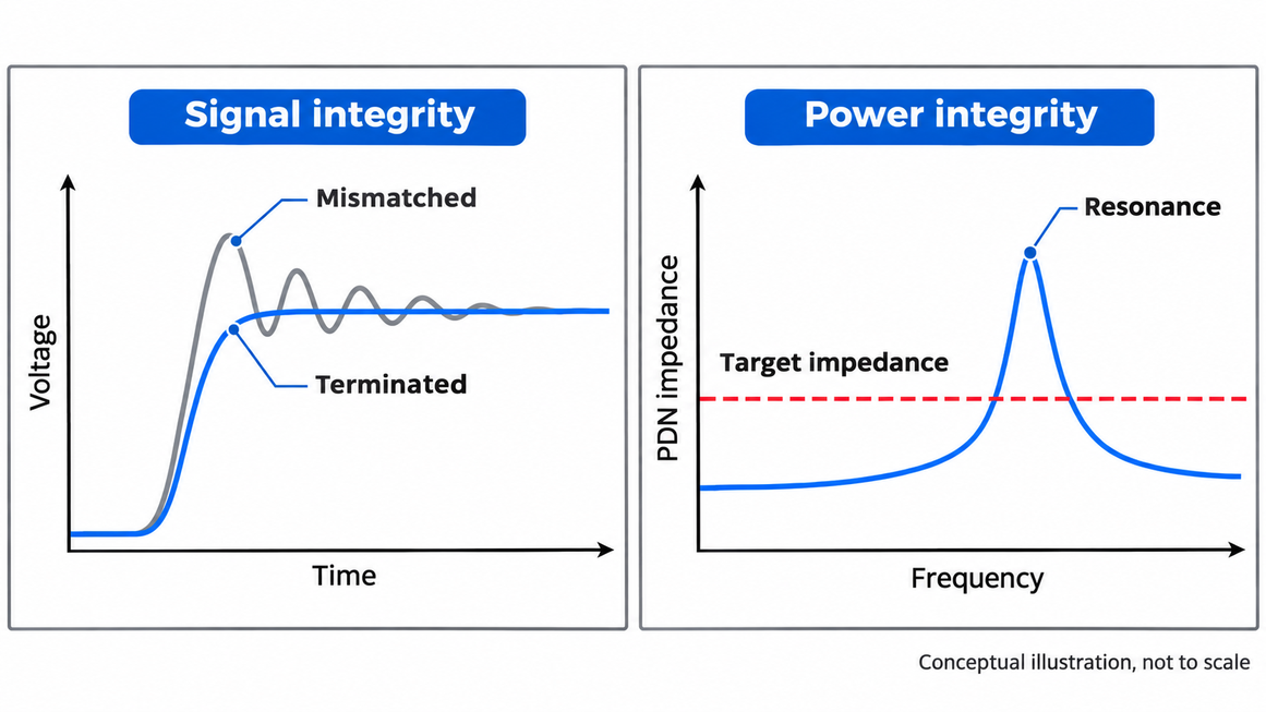
Figure 4: Ringing from an impedance mismatch and PDN impedance against its target
Power integrity simulation involves analyzing the power distribution network (PDN), comprising power planes, vias, and capacitors, that supplies each IC. DC analysis can chart the current density and voltage drop across the copper, alerting before a narrow plane neck kills a processor core. The AC analysis is performed by comparing the design's PDN impedance with the target impedance, which is the ripple voltage/target current at each frequency. In this case (0.9 V rail, 5% ripple, 15 A transient), the target is 3 mΩ.
Thermal and Multiphysics Analysis for Heat Management
Thermal simulation predicts where heat collects and how hot each component runs. The laminate is a poor conductor: an FR-4-class material such as Isola 370HR conducts about 0.4 W/m·K, whereas copper conducts roughly 1,000 times as well. Heat from a regulator or power MOSFET therefore spreads along copper planes and down through thermal vias, and the simulation shows whether those paths keep each junction inside its rating.
Multiphysics analysis couples heat with another physical domain. The common case is electro-thermal. Copper resistance increases by about 0.4% per °C, so a hot plane drops more voltage, dissipates more power, and heats up further. The solver therefore iterates the electrical and thermal results until they settle. Airflow models add the enclosure and fans. Mechanical models then use the temperature map to estimate warpage and solder joint stress where materials expand at different rates.
Electromagnetic Compatibility for Noise Control
EMC simulation estimates how much a board radiates and how easily outside fields disturb it. Most emission problems come from current loops. At high frequencies, return current flows in the reference plane directly under its signal trace, because that path has the lowest inductance. A trace that crosses a split in the plane forces the return current around the gap, and the enlarged loop radiates like a small antenna.
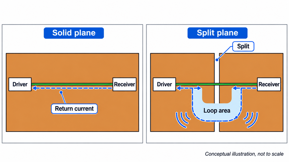
Figure 5: Return current under a trace on a solid plane and around a split
Simulation finds these structures before a test lab does: plane splits under fast nets, clock routes near board edges, and connectors with a poor ground return. It cannot certify a product because emission limits are met or exceeded in a measured test with the actual enclosure and cables. Its value is ranking the risks, so the layout fixes from EMC design practice go where they matter before the first compliance scan.
Turn Simulation Results into a Manufacturing-Ready PCB
A simulation is valid only for the board it models, so three checks ensure the fabricated board has the stackup, geometry, and tolerances assumed by the analysis.
Review Stackup, Impedance, and Copper Geometry
The field solver needs the same inputs the fabricator will use to build: trace width, copper thickness, dielectric height to the reference plane, the dielectric constant (Dk) of each prepreg and core, and the solder mask over the outer traces. If the model and the board differ in any one of them, the result moves. Prepreg Dk varies with glass style and resin content, so a stackup modeled with one generic FR-4 value will not match a board pressed from specific prepregs.
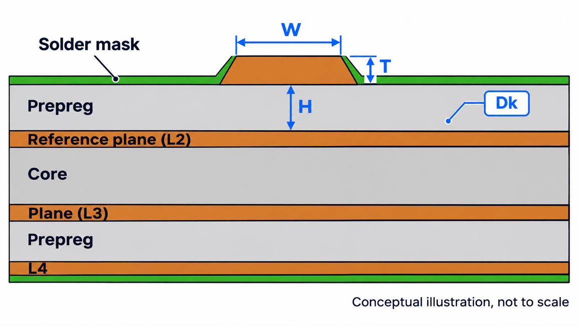
Figure 6: Stackup inputs a field solver needs to match the fabricated board
Two more details shift the answer. Etched traces are trapezoidal, narrower at the top than at the base, and outer-layer copper is typically plated thicker than its base foil. On multi-gigabit links, copper roughness and the fall in Dk with frequency add loss and move impedance further. So build the model from the fabricator's published stackup. Rerun the impedance control calculation whenever a layer or copper weight changes, and tag every controlled net with its target.
Check Design Rules Against Real Fabrication Limits
A design which appears to be able to build a well can still be unbuildable. Upload the Fabricator's limits to the layout tool's design rule check before routing. The minimum trace width and spacing for each copper weight, the minimum drill and via sizes, the annular ring, and the hole-to-copper clearance are the key parameters. These limits interact with the simulation. The heavier the copper, the less DC drop in a power plane, and the wider the minimum trace and spacing. A low-bandwidth controlled-impedance trace may also be below the ability of the fabricator to etch the trace on that layer.
Wherever the layout allows, use recommended values rather than absolute minimums. Etch variation is held fairly constant in absolute terms; that is, a line of minimum width will have a higher impedance variation than a wider line over a greater thickness of dielectric. Redo design rule check after each change made based on a simulation, as widening a plane neck or adding stitching vias for a particular clearance may cause it to fail the check.
Prepare Fabrication Data and Verify Critical Requirements
The fabrication package carries the simulation's assumptions to the manufacturer. Gerber or ODB++ files, or an IPC-2581 data set, define the copper and drill geometry, but the requirements behind that geometry belong in the fabrication drawing and order notes, each traced to the analysis that set it.
| Simulation Result | Fabrication Requirement | Where It Is Stated |
|---|---|---|
| Impedance model and trace widths | Stackup, dielectric heights, Dk, copper weights | Stackup drawing or stackup selection |
| Signal integrity on controlled nets | Target impedance, tolerance, layer, reference plane | Fabrication drawing notes |
| DC drop and thermal results | Copper weight per layer, thermal via structure | Stackup drawing and drill data |
| Mechanical and stackup fit | Finished board thickness and tolerance | Order notes |
Before release, compare each row with the simulation report and the fabricator's capability. A mismatch found here costs an edit, while the same mismatch found on a prototype costs the whole build.
How JLCPCB Capabilities Support Simulation-Driven Designs
A simulation-driven design needs a fabricator whose stackups, materials, and tolerances are published, so the model can start from what will be built.
Multilayer and Controlled-Impedance PCB Manufacturing
JLCPCB builds boards from 1 to 32 layers and offers impedance control on multilayer boards. The standard tolerance is ±10%; ±5% is available upon special request. For 4- and 6-layer boards, it lists named impedance stackups, such as JLC04161H-7628, with the prepreg, core, and copper of each, and states that the board is produced to the selected stackup.
That gives the field solver fixed inputs. Choose the stackup first, then enter its dielectric heights and Dk values into the simulation. The impedance calculator gives trace widths for each target impedance on that build. When the critical nets are simulated with those widths, the model and the fabricated board start from the same numbers.
Material and PCB Structure Selection
Material choice sets the inputs for both the electrical and the thermal model. The same capabilities page lists Grade A FR-4 from suppliers including Nan Ya, KB, and Shengyi, along with the dielectric constants and impedance or crosstalk model needs.
| Material Option | Published Values | Simulation Use |
|---|---|---|
| FR-4 prepreg 7628 / 3313 / 2116 / 1080 | Dk 4.4 / 4.1 / 4.16 / 3.91 | Dielectric layers in impedance and crosstalk models |
| FR-4 core | Dk 4.6 | Inner-layer dielectric |
| Solder mask | Dk 3.8, ink thickness 10 µm or more | Outer-layer microstrip impedance |
| Rogers and PTFE cores | 2-layer RF boards, 1 oz copper | Low-loss RF lines |
| Aluminum and copper core | 1-layer boards | Heat spreading for power and LED boards |
Structure choices follow the simulation results. Multilayer boards take 1 or 2 oz outer copper and 0.5, 1, or 2 oz inner copper, so a PI result that calls for heavier inner planes fits a standard build. Heavier copper raises the etching limit, though: on a 2-layer board, minimum trace and space rise from 0.10 mm (4 mil) at 1 oz to 0.16 mm (6.5 mil) at 2 oz.
From Design Verification to Fabrication
The hand-off is short when the simulation uses the fabricator's own values. Select impedance control and the named stackup on the order, so the board is pressed to build the model assumed. State the finished thickness in the order notes. JLCPCB recommends sending the stack-up diagram for engineering review before ordering boards with more than 10 layers. Advanced options typically require a DFM review, which can add cost and time.
A prototype then confirms the results on real hardware: measured rail ripple, eye openings, temperatures, and a pre-compliance emissions scan. When those agree with the simulation, the model is calibrated for the next revision. Upload your Gerber files to get an instant quote for that first build.
FAQs about PCB Simulation
Q: Is PCB simulation necessary for every board?
No. A low-speed, low-current board with relaxed timing often needs only circuit simulation and a design rule check. Signal integrity, power integrity, thermal, and EMC simulations are worth the time when edge rates are fast, rails carry high current, parts run hot, or the product must pass emissions testing.
Q: What software is used for PCB simulation?
SPICE engines such as ngspice and LTspice handle circuit simulation and are often built into schematic editors. Signal integrity, power integrity, thermal, and EMC work use field solvers, either inside PCB design suites or in dedicated simulation packages.
Q: What is the difference between SPICE and IBIS models?
A SPICE model describes a component's internal circuit, so it is detailed but slow and can expose proprietary design. An IBIS model describes only an I/O buffer's behavior at its pins via current-voltage and voltage-time tables, making it fast enough for board-level signal-integrity simulation.
Q: Can PCB simulation replace prototype testing?
No. Simulation reduces the number of prototypes by identifying geometry-driven problems early, but its accuracy depends on the models and inputs used.
Q: What is the difference between signal integrity and power integrity?
Signal integrity concerns the quality of signals traveling along traces: reflections, crosstalk, and timing. Power integrity concerns the supply voltage that drives them: DC drop and noise on the power distribution network.
Conclusion
PCB simulation prevents the following geometry-related issues: impedance mismatches, supply droop, hot spots, and radiating return paths. It does not catch footprint errors or assembly defects, and it is valid only when the model matches the built board. The decision rule is to simulate any layout change that could fix it, using the fabricator's stackup, Dk values, and limits as inputs, and then confirm on the prototype.
When the design and its fabrication notes agree, order your PCBs from JLCPCB with the stackup your simulation used.
Popular Articles
Keep Learning
Design Guide for USB-3.0 Differential Signaling
In the world of data transfer, USB 3.0 is the Usain Bolt to USB 2.0’s friendly jogger. USB 2.0 is called “High Speed” and limped along at 480 Mb/s, whereas USB 3.0 SuperSpeed rockets up to 5 Gb/s (over ten times faster). But this speed jump brings full‑duplex operation and new differential transmit (SSTX) and receive (SSRX) pairs on dedicated pins. USB 2.0 D+/D– lines handle enumeration and legacy data, while two new 5 Gb/s high‑speed differential pairs carry SuperSpeed data in each direction. While m......
Can PCB Simulation Prevent Costly Manufacturing Revisions?
Key Takeaways PCB simulation identifies electrical, thermal, and EMC issues before fabrication, helping reduce costly design revisions. Signal integrity, power integrity, thermal, and EMC analysis address different PCB performance risks. Accurate simulation depends on matching the model to the actual stackup, materials, and manufacturing limits. Combining simulation with DRC checks and prototype testing helps ensure reliable, manufacturable PCB designs. PCB simulation is the practice of predicting how......
EMC Design for PCB: EMI, EMS, Testing Standards & Compliance Guide
Key Takeaways EMC design means controlling both EMI (unwanted emissions) and EMS (immunity to external disturbances); a board that meets emission limits but resets during an ESD test has not achieved EMC. Every interference problem can be analyzed with the source–path–victim model, and solved by reducing the source, interrupting the path, or hardening the victim. Core PCB techniques include minimizing current-loop area, maintaining continuous reference planes, controlling impedance, decoupling power p......
How to Choose and Place Decoupling Capacitors for PCB Design
Every digital PCB depends on decoupling capacitors, yet a surprising number of boards still suffer from voltage dips, glitches, and electromagnetic interference (EMI) issues caused by one simple mistake: incorrect placement or selection. This guide walks through what decoupling capacitors do, how to choose the right value, where to place them, and which layout mistakes to avoid, so your next board runs clean on the first try. Key Takeaways Place one decoupling capacitor near each IC's power pin. Use 1......
Effective Solutions to Reduce PCB Ground Loop Noise
Key Takeaways Cause: Multiple ground paths with voltage differences cause hum, ADC errors, and EMI. Strategy: Use star grounding for <1 MHz; use solid ground planes for >10 MHz. Routing: Never route fast traces across split planes to avoid large return loops. Mitigation: Use isolation, differential pairs, and place GND vias/caps close to IC pins. Stackup: Use thinner prepreg to lower return loop inductance. A ground loop occurs when multiple grounds form a closed conductive path, allowing unwanted ele......
Building Effective ESD Protection Into PCB Design
Key Takeaways Layout Rules: ESD spikes rise in nanoseconds; routing layout matters more than part specs alone. Clamp First: Place TVS diodes right at the connector using direct, flow-through traces. Low-Inductance Ground: Use short, wide traces with immediate ground vias to prevent voltage shifts. Capacitance Limits: Use low-capacitance clamps (< 0.5 pF) on high-speed lines like USB 3.x. DFM-Ready: Account for standard via and trace tolerances to ensure reliable board fabrication. ESD protection on a ......