Managing Skin Effect Loss in High-Frequency PCB Design
17 min
- Understanding Skin Effect in High-Speed PCBs
- Key Factors Increasing Skin Effect Losses
- How to Reduce Skin Effect in PCB
- Our Manufacturing Solutions for High-Frequency PCBs
- FAQs About Skin Effect
- Conclusion
Key Takeaways
- Skin Depth Shrinks: High frequencies force current to the trace surface, shrinking depth to 0.66 µm at 10 GHz.
- Roughness Adds Loss: Copper foil roughness lengthens current paths, sharply increasing high-speed resistance.
- Plating Affects Signals: Low-conductive finishes like ENIG nickel increase attenuation on exposed lines.
- Wider Traces Help: Wider traces and thicker dielectrics lower conductor loss by expanding current surface area.
- Use Smooth Foils: Pairing low-profile copper foils (VLP/HVLP) with advanced laminates is essential for 10+ GHz designs.
Skin effect pushes high-frequency current into a thin layer at the surface of a copper trace. The trace then behaves as if most of its copper were missing. At 1 GHz, that layer is only about 2 µm deep, while a standard 1 oz trace is 35 µm thick. A changing current builds a changing magnetic field inside the conductor. That field induces small opposing currents in the middle of the copper, which cancel flow in the core and reinforce it near the surface.
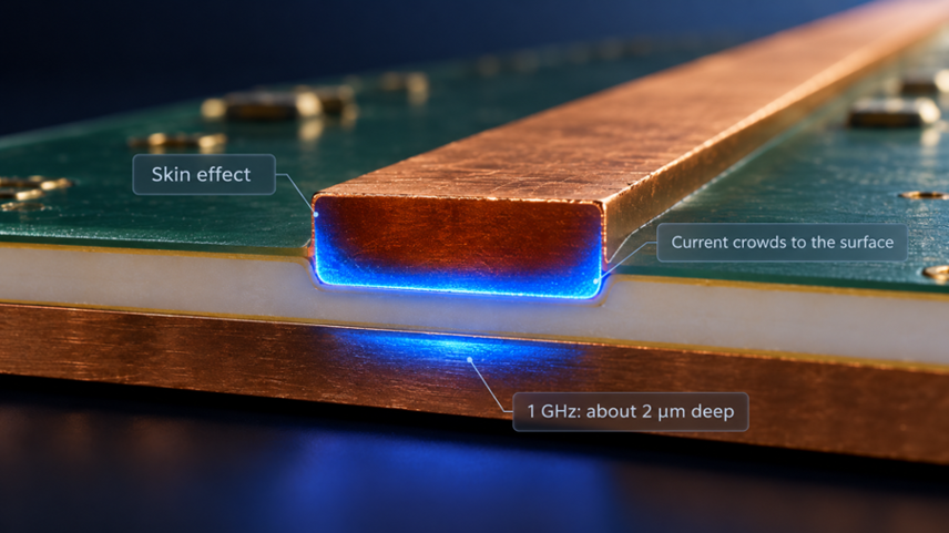
Figure 1: Skin effect concentrating current in the outer layer of a PCB
The quicker the signal changes, the shallower the band that it can utilize. At this point, the thickness of the copper and which metal is being plated over it determine how much signal will get through. In this guide, skin depth is explained, and how foil roughness and surface finishes contribute to loss. It then demonstrates how copper, trace geometry, and laminates can be selected to ensure that high-frequency loss is affordable.
Understanding Skin Effect in High-Speed PCBs
Skin effect is found in all conductors having alternating current. On a PCB, it is a rule that determines how much copper a fast signal can use. This, in turn, determines the loss the line contributes.
What Is Skin Effect and Skin Depth?
Alternating current tends to flow more on the surface of a conductor than in the entire cross-section of the conductor. The skin depth is the depth below the surface of the material at which the current density is approximately 37% of the current density at the surface. About 63% of current flow is within that initial skin depth, and that is considered to be the useful thickness of the conductor, so that is what engineers consider to be the “skin depth.”
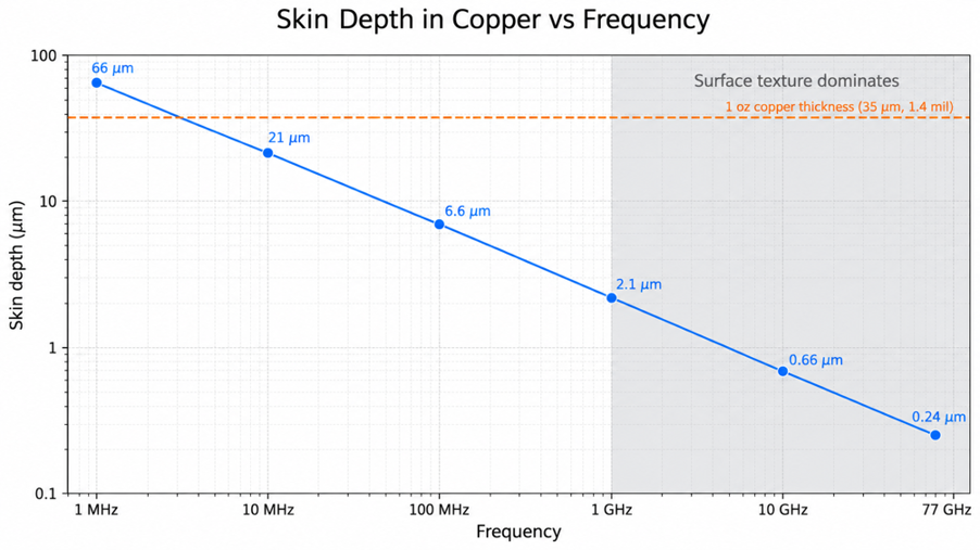
Figure 2: Copper skin depth versus frequency from 1 MHz to 77 GHz
Skin depth is related to the electrical resistivity of the conductor, the signal frequency, and the material's magnetic permeability. It is computed based on:
δ = √[ρ / (π f μ₀ μᵣ)]
Where:
- δ = Skin depth (m)
- ρ = Electrical resistivity of the conductor (Ω·m)
- f = Signal frequency (Hz)
- μ₀ = Permeability of free space (4π × 10⁻⁷ H/m)
- μᵣ = Relative magnetic permeability of the conductor (approximately 1 for copper)
δ ≈ 66 / √f₍MHz₎ µm
Here, f is given in megahertz (MHz), and δ is given in micrometers (µm). As frequency increases, skin depth decreases. For example, copper has a skin depth of approximately 66 µm at 1 MHz and 6.6 µm at 100 MHz.
| Frequency | Skin Depth in Copper | Where You Meet It | What It Means for a 1 oz (35 µm, 1.4 mil) Trace |
|---|---|---|---|
| 1 MHz | 66 µm (2.6 mil) | Switching regulator loops | Current still fills the full thickness |
| 10 MHz | 21 µm (0.82 mil) | Slow clocks and their harmonics | The center of the trace starts to empty |
| 100 MHz | 6.6 µm (0.26 mil) | Fast digital edges | Less than a fifth of the thickness carries current |
| 1 GHz | 2.1 µm (0.08 mil) | Gigabit serial links | Surface texture begins to matter |
| 10 GHz | 0.66 µm (0.026 mil) | Multi-gigabit links, X-band RF | Foil roughness dominates conductor loss |
| 77 GHz | 0.24 µm (0.009 mil) | Automotive radar | Only the outermost skin of the copper conducts |
How High-Frequency Current Moves in Copper
When current flows in a trace, it will redistribute because the trace and the return path are in a loop that does not like magnetic flux changes. Resistance is the only hindrance at low frequencies, and current is uniform. At high frequencies, the reactance of inductance predominates, and the current flows through the path with the smallest flux. These are the paths that are closest to the return current in the plane.
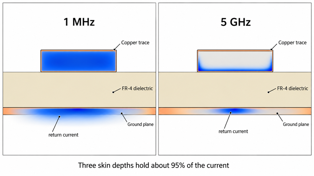
Figure 3: Current density in a microstrip cross-section at 1 MHz and at 5 GHz
Current thus concentrates on the lower surface of the microstrip trace and at the two lower corners of the microstrip. It is mirrored in a thin strip of plane under the trace by the return current. During this process, the electric field around the trace does not change, and thus the skin effect does not affect the line capacitance. Only the present concentration in the subsurface is changed. This slightly increases the trace's resistance and decreases its internal inductance.
Impact on Signal Attenuation and Integrity
Because of the skin effect, the trace's resistance increases with frequency, dissipating signal energy as heat. In the case of a smooth copper transmission line, Eric Bogatin has estimated the conductor attenuation as:
Conductor loss (dB/in) ≈ [36 / (w × Z₀)] × √f₍GHz₎
Where:
- w = Trace width in mils (1 mil = 0.001 in)
- Z₀ = Characteristic impedance of the line (Ω)
- f₍GHz₎ = Signal frequency in gigahertz (GHz)
- Conductor loss = Approximate attenuation in decibels per inch (dB/in)
For a 5 mil (0.127 mm) wide, 50 Ω line at 10 GHz:
Conductor loss ≈ [36 / (5 × 50)] × √10 ≈ 0.46 dB/in
Skin effect loss is frequency-dependent and affects the integrity of the signal. A digital edge is composed of a multitude of harmonics, and the skin effect takes off more from the higher harmonics than from the lower harmonics. As the edge propagates through the rise time, each bit “smears” into the next, and the eye diagram closes at the receiver.
Key Factors Increasing Skin Effect Losses
The metal and the frequency determine the skin depth. However, the amount of loss it creates depends on the current that flows through that thin band. Each change that results in loss is related to the surface texture, geometry of the dielectric, and the amount of plated metal.
Copper Foil Surface Roughness
The side of the copper foil that attaches to the laminate is roughened. The tooth structure secures it to the resin, providing peel strength to the board. In a microstrip, the treated side is the side facing the ground plane, where the current is concentrated. When the roughness is near the skin depth, the current follows all the peaks and valleys, and the path length and resistance increase.
The Hammerstad roughness correction is used for the extra conductor loss due to a rough copper surface. It is regarded as acting as a multiplying factor proportional to the frequency of the estimated loss for smooth copper:
Kᵣ = 1 + (2/π) × arctan[1.4 × (Δ/δ)²]
Where:
- Kᵣ = Roughness correction factor (dimensionless)
- Δ = RMS copper surface roughness (µm)
- δ = Skin depth at the signal frequency (µm)
- arctan = Inverse tangent function (in radians)
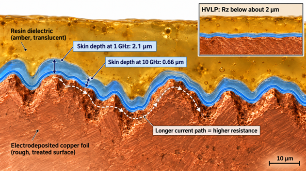
Figure 4: Rough copper foil profile compared with skin depth at 1 GHz and 10 GHz
The correction factor for copper foil with an RMS roughness of 1 µm (about 0.04 mil) is ~1.20 at 1 GHz. This rises to about 1.81 at 10 GHz. Therefore, the conductor loss for the same rough copper surface (at 10 GHz) is approximately 81% higher than the smooth-copper estimate. The model is an approximation, and actual behavior will depend on the copper profile and the geometry of the transmission line.
Plating Materials and Surface Finishes
Surface finish is merely copper that is exposed by the solder mask, for example, pads, edge launches, and not masked RF lines. On those surfaces, the finish is the skin, and a metal with a lower conductivity than copper introduces loss:
- ENIG deposits 3-6 µm (0.12-0.24 mil) of electroless nickel under approximately 0.05 µm (2 µin) of gold, and nickel conducts several times better than copper.
- HASL is a tin-based solder that coats the copper, has a conductivity of about 1/8 that of copper, and varies in thickness.
- OSP is an organic coating on bare copper; therefore, no penalty for using the current.
- Using immersion silver leaves behind a thin film of the most common conductor, and its impact on loss is almost null.
ENIG is critical at high frequencies, such as multi-gigahertz, because at these frequencies, currents penetrate only a few micrometers. A lot of the current on an ENIG surface flows through the nickel, and the 3 to 6 µm thick layer of nickel fills that band.
Dielectric Materials and Trace Geometry
The dielectric will not cause skin effect, but does determine the width of the trace. Width, in turn, determines the extent of the surface area that the current can flow over. The narrower the distance between the target and the trace, the higher the dielectric constant or the thinner the dielectric, which will push the trace to be narrower for a given target of 50 Ω. Conductor loss is approximately proportional to 1/w; therefore, a narrow width will approximately double the resistance per inch.
When you etch, that width is even smaller, since the etchant works top-down, leaving the laminate with a trapezoidal shape, with the wider foot on the laminate. The majority of the current flow on a micro strip is carried by that foot. So, the width lost due to etching is lost from the busiest copper, and that is why impedance control for PCB design and loss control are the same discipline.
How to Reduce Skin Effect in PCB
When the frequency is constant, the skin depth is unchanged; therefore, reducing skin-effect losses means providing a smoother, wider, better-conducting surface. The three levers are associated with the three causes: foil, geometry, and laminate.
Choosing Low-Roughness Copper Foils
The reason for selecting foil as the laminate is that the copper is bonded to the core during laminate manufacturing. Most suppliers offer a range of foil grades for each core, with smoother grades priced higher. The copper foil specification (IPC-4562B) defines profile classes, and the roughness is specified in the datasheet as Rz, the peak-to-valley height.
| Foil Type | Typical Treated-Side Rz | Compared with 10 GHz Skin Depth (0.66 µm) | Where It Fits |
|---|---|---|---|
| Standard ED | 7 to 10 µm (0.28 to 0.39 mil) | More than 10 times deeper | Power, control, and digital below about 1 GHz |
| Reverse treated (RTF) | About 3 to 6 µm (0.12 to 0.24 mil) | 4 to 9 times deeper | High-speed digital in the low gigahertz |
| Very low profile (VLP) | 3 to 5 µm (0.12 to 0.20 mil) | 4 to 8 times deeper | 5 to 10 Gbps links and sub-6 GHz RF |
| Hyper very low profile (HVLP) | Below about 2 µm (0.08 mil) | Up to 3 times deeper | 25 Gbps and faster links, millimeter-wave RF |
After 10 GHz, harmonics are energetic, and only VLP, HVLP, and the smoothest RTF grades are rough by only a few skin depths. For RTF, since it has no IPC roughness class, refer to its Rz on the datasheet.
Optimizing Trace Width and Thickness
The most powerful geometry lever is width, as conductor loss is proportional to the width of the current-carrying face to a good approximation. The wider the trace, the greater the dielectric height required to support 50 Ω.
- Set the target impedance (e.g., 50 Ω single-ended or 100 Ω differential).
- Pick the thickest dielectric to the reference plane that the stackup will provide.
- Measure the width of the trace at that height; it will be larger than the default width.
- Do not tightly couple differential pairs, as this results in narrow 100Ω traces.
The thickness of the copper is of little consequence at gigahertz frequencies, since the 1 oz trace is 35 µm (1.4 mil) thick, which is about 17 skin depths at 1 GHz. There's no change there, and JLCPCB's minimum spacing for 2 layers is increased to 0.16 mm (6.5 mil) with a switch to 2 oz. The skin depth is still similar to the thickness of copper, and thicker copper will only help below about 15 MHz. On top of that, invest in width and impedance-controlled routing.
Selecting Advanced Board Materials
A low-loss laminate reduces dielectric loss directly, making conductor loss the larger share of the total.
Bogatin’s approximation estimates dielectric insertion loss per unit length using the dissipation factor and dielectric constant:
Dielectric loss (dB/in) ≈ 2.3 × f₍GHz₎ × Df × √Dk
Where:
- f₍GHz₎ = Signal frequency in gigahertz (GHz)
- Df = Dielectric dissipation factor (loss tangent), dimensionless
- Dk = Relative dielectric constant, dimensionless
- Dielectric loss = Approximate attenuation in decibels per inch (dB/in)
This estimate is approximately twice the stated copper conductor loss for a 5-mil trace. Actual loss depends on the laminate properties, trace geometry, and frequency.
On RO4350B, with Dk 3.48 and Df 0.0037, the same formula gives 0.16 dB per inch. Copper then accounts for about three-quarters of the loss, so pairing a premium laminate with rough foil largely wastes its benefit. That is why Rogers offers RO4350B LoPro with reverse-treated foil.
| Application | Signal Band | Recommended Laminate | What This Means for Skin Effect |
|---|---|---|---|
| Control, USB 2.0, SPI | Below 1 GHz | Standard FR-4 | Standard foil is fine, and conductor loss stays small |
| PCIe Gen 3, 10G Ethernet | 4 to 5 GHz Nyquist | Mid-loss FR-4 family | Specify VLP or RTF foil on the fast layers |
| Wi-Fi, 5G sub-6 GHz RF | 2.4 to 6 GHz | RO4350B or similar | Pair with low-profile foil and keep RF lines short |
| Radar, mmWave links | 24 to 81 GHz | PTFE-based laminate | Smooth foil and a non-nickel finish on exposed lines |
Our Manufacturing Solutions for High-Frequency PCBs
A low-loss design remains low-loss given that the factory reproduces the model width, copper, and finish. JLCPCB's high-frequency and impedance-controlled services cater to all those inputs.
Precise Copper Etching and Roughness Control
The width of the traces is determined at imaging and etching; thus, the accuracy of this width is dependent on the accuracy of the pattern exposure. JLCPCB operates fully automatic laser direct imaging lines that write the pattern directly from your data without using a film phototool. The low-loss lines require a wide geometry, which is met by the standard capability of 0.10 mm (4 mil) trace and space on 1 oz copper.
At JLCPCB, it depends on the material choice because the laminate determines the level of roughness. The high-frequency PCB service can fabricate 2-layer, 1 oz boards based on the Rogers RO4350B/ZYF-series PTFE laminate with Df as low as 0.0016. These laminates do not have a foil profile listed in the capability pages. If the loss model requires VLP or HVLP copper, verify the foil grade with support before specifying the stackup to verify that the board is modeled correctly.
High-Speed Surface Finish Capabilities
Conventional rigid boards are available with HASL (leaded or lead-free), ENIG, and OSP. On a high-speed FR-4 Board with Exposed Transmission Lines, OSP maintains current in bare copper without a conductor penalty. When exposed copper is limited, the choice is often ENIG since it is usable for fine-pitch BGAs and connectors that require flat pads.
The high-frequency line is supplied with ENIG at 1 or 2 µin (approximately 0.025 or 0.05 µm) of gold. Thin gold has virtually no flow of RF current, and the nickel underneath determines the loss on each surface that is exposed. Wherever possible, keep long RF lines under your solder mask, per your impedance model. Add that mask to that model, as it reduces the impedance by a couple of ohms.
Strict Impedance and Signal Testing
With impedance control enabled in the order, JLCPCB offers impedance with a standard tolerance of ±10% on multilayer boards and a special tolerance of ±5%. The JLCPCB impedance calculator is based on the actual stackups used in those orders; therefore, the width value it provides is the width the process expects. Each order with impedance control is TDR-tested around the panel border in accordance with the PCB impedance testing in the TDR guide.
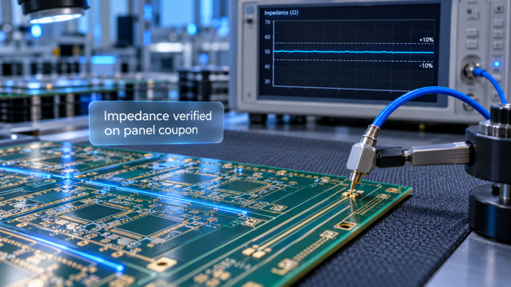
Figure 5: TDR impedance testing on a PCB test coupon at the panel border
TDR confirms impedance only and not insertion loss. Add the straight test line and check for skin-effect loss in the first batch using a vector network analyzer. Gerber files and impedance control can be enabled on JLCPCB's quote page.
FAQs About Skin Effect
Q: Does skin effect matter on a 50 MHz SPI bus?
Only slightly. Skin depth at 50 MHz is about 9 µm, so the current uses part of a 1-oz trace, and resistance rises. Runs are short, though, so reflections and crosstalk cause problems long before skin effect does.
Q: Can I use 2 oz of copper to reduce skin effect?
Not above about 15 MHz. Once skin depth is far thinner than the copper, extra thickness carries no current, so 2 oz only adds cost and wider spacing. A wider trace or smoother foil reduces the loss far more.
Q: Is skin effect the same as proximity effect?
No, but they act together. Skin effect pushes current to the surface of one conductor, while proximity effect pulls it toward a nearby conductor carrying the opposite current. That is why current crowds onto the trace face nearest the reference plane.
Q: Would silver-plated traces remove skin effect loss?
No. Silver conducts only about 6% better than copper, and skin effect resistance scales with the square root of resistivity, so the gain is roughly 3%. Smoother foil helps far more, since roughness can nearly double the resistance.
Q: Why is my measured loss higher than the simulation?
Most simulators assume smooth copper unless you enter a roughness model. Add the foil profile from the laminate datasheet using the Hammerstad or Huray model. Include any ENIG surface on exposed lines, too, because both raise loss above the smooth estimate.
Conclusion
Skin effect is not a fault to be avoided, as all the high-speed signals in a PCB will experience it. You control the surface on which the current is pushed. At low frequencies, the resistance is determined by the copper thickness. At gigahertz rates, it is left to the foil roughness, the finish on the exposed copper, and the trace width on the dielectric to determine the choice.
Skin depths continue to scale down below the thickness of standard foil as link rates climb past 112 Gbps per lane into deeper millimeter-wave bands. The foil grade will be shown on the stackup drawing next to Dk and Df, rather than in a footnote. Once the design is complete, you can put your design options to the test on real hardware using JLCPCB's impedance-controlled and Rogers or PTFE high-frequency boards.

Popular Articles
Keep Learning
Getting PCB Characteristic Impedance Right for Reliable Signals
Key Takeaways Impedance Defined: Characteristic impedance is set by trace geometry and the reference plane, not by copper DC resistance. Core Factors: Trace width, copper thickness, dielectric height, and dielectric constant determine the impedance value. Reference Plane: High speed traces need a continuous reference plane to prevent signal reflection. Factory Verification: Fabricators adjust trace width and check impedance using time domain reflectometry on test coupons. Design Approach: Select a sta......
Managing Skin Effect Loss in High-Frequency PCB Design
Key Takeaways Skin Depth Shrinks: High frequencies force current to the trace surface, shrinking depth to 0.66 µm at 10 GHz. Roughness Adds Loss: Copper foil roughness lengthens current paths, sharply increasing high-speed resistance. Plating Affects Signals: Low-conductive finishes like ENIG nickel increase attenuation on exposed lines. Wider Traces Help: Wider traces and thicker dielectrics lower conductor loss by expanding current surface area. Use Smooth Foils: Pairing low-profile copper foils (VL......
Stop PCB Crosstalk Before It Becomes a Signal Integrity Problem
Key Takeaways NEXT vs FEXT: NEXT saturates with trace length, while FEXT grows linearly with distance. Spacing & Stackup: Apply the 3W rule and keep traces close to reference planes. Edge Rates: Fast rise times drive crosstalk more than clock frequency. Fab Margins: Etching variations reduce gaps, requiring extra layout clearance. Verification: Use DFM checks and TDR coupons instead of basic continuity tests. PCB crosstalk is the noise one trace pushes into its neighbor, even though the two nets are e......
Navigating the Impedance Landscape: Selecting the Right Impedance for USB, Ethernet, HDMI, and SD Card Interfaces
Introduction In the realm of high-speed digital communication, choosing the right impedance is a critical aspect of successful PCB design. Impedance matching ensures optimal signal integrity, minimizes reflections, and enhances the overall performance of interfaces such as USB, Ethernet, HDMI, and SD Card. In this blog post, we'll explore the importance of impedance, the factors influencing impedance selection, and best practices for ensuring reliable data transmission in these widely used interfaces.......
A Beginners Guide to Impedance Control in PCBs
When a digital signal is transmitted from one point to another, it causes a change in the state of the signal line. This change can be understood as an electromagnetic wave moving through the circuit. Reflection occurs when this wave encounters a boundary between different mediums. At this boundary, some of the wave's energy continues as a signal, while the rest is reflected. This process repeats until the energy is either absorbed by the circuit or dissipated into the environment. For electrical engi......
What is PCB Signal Attenuation: How Signals Weaken Over Distance and How to Mitigate It
Key Takeaways Primary Causes: Signal attenuation is mainly caused by skin effect (conductor loss) and substrate energy absorption (dielectric loss). How to Mitigate: Reduce loss by using wider traces, low-loss materials, controlled impedance, and removing via stubs. JLCPCB Solutions: JLCPCB offers Rogers high-frequency laminates, High-TG FR4, precision impedance control, and backdrilling to protect signal integrity. As a signal travels from the source to the load through PCB conductors, the signal is ......