
Modeling Induction Heating Without Guesswork: From Maxwell's Equations to Practical Simulation Workflows
10 min
- Why Simulation is Essential in Induction Heating
- The Physics: A Primer on Maxwell's Equations
- A Primer on Vector Operators
- Constitutive Relations and Material Properties
- Practical Simplifications for Engineers
- Choosing the Right Numerical Method
- Model Credibility Checklist
- FAQ about Induction Heating Simulation
Key Takeaways
Simulation over prototyping: Mathematical modeling eliminates costly trial-and-error by predicting how nonlinear factors affect thermal outcomes before production.
Maxwell's equations are the foundation: Ampere's and Faraday's Laws govern how alternating coil currents induce eddy currents in the workpiece, defining the core physics of induction heating.
Choose the right numerical method: FEM excels at complex geometries, BEM/MIM reduce mesh size for elongated systems—no single method fits every application.
Know when to include hysteresis: For high-temperature processes above Curie, hysteresis is negligible; for low-temperature applications like tempering or curing, it must be modeled.
Why Simulation is Essential in Induction Heating
Simulation is more than just a digital replica of a physical process; it is a predictive tool that captures how interrelated and nonlinear factors affect the transitional and final thermal conditions of a component. For instance, when designing a new heat treatment process, simulation helps determine exactly what must be accomplished to improve effectiveness and establish appropriate process recipes. Without it, engineers are often left guessing how a change in frequency or coil geometry might affect the skin effect or the Curie-point transition in magnetic steels.
However, mathematical modeling is not a "magic button." The quality of the results is strictly derived from the governing equations and the assumptions made by the analyst. Before starting a simulation, a sound understanding of the nature and physics of the process is necessary. Engineers must be aware of the limitations of their models and the sensitivity of the results to poorly defined parameters. Common pitfalls include inaccurate boundary conditions, uncertain material properties, and oversimplified assumptions about initial temperature distributions. Choosing the right theoretical model—ranging from simple hand-calculated formulas to complex numerical analyses—requires balancing complexity, accuracy, time limitations, and cost.
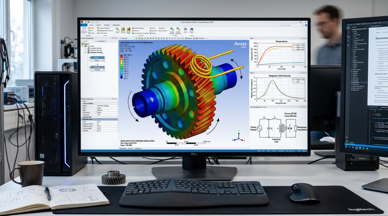
A modern engineering workstation utilizing advanced simulation software to visualize the coupled electromagnetic and thermal effects on a gear during induction heating.
The Physics: A Primer on Maxwell's Equations
The core of any induction heating simulation is the ability to solve Maxwell's equations. These equations describe the behavior of electromagnetic fields in their differential form:
- Ampere's Law: States that the curl of the magnetic field intensity (H) has two sources: conduction current density (J) and displacement current density. In the context of induction heating, this equation suggests that a magnetic field is produced whenever electric currents flow in surrounding objects.
- Faraday's Law: Shows that a time-varying magnetic flux density (B) produces a curling electric field (E) and induces currents in the surrounding area. The minus sign in this equation is critical as it determines the direction of the induced electric field.
- Gauss' Law for Magnetism: Indicates that the divergence of magnetic flux density is zero. This means that magnetic flux lines have no source or sink points; they always form continuous loops.
- Gauss' Law for Electricity: Relates electric flux density (D) to the electric charge density.
Physical Interpretation in Induction Heating
When we apply alternating voltage to an induction coil, an alternating current (AC) appears in the circuit. According to Ampere's Law, this alternating coil current produces an alternating magnetic field in its surroundings at the same frequency. This field's strength depends on the coil current magnitude, geometry, and coupling with the workpiece. As Faraday's Law describes, this changing magnetic field induces eddy currents in the workpiece. Crucially, the minus sign dictates that these induced currents flow in a direction opposite to that of the coil current.
These alternating eddy currents then produce their own magnetic fields, which also have opposite directions to the main magnetic field of the coil. The total magnetic field is the product of these interacting source and induced fields. Analysts must be cautious: Ampere's Law also suggests that undesirable heating can occur in any electrically conductive structures located near the coil, such as tools, fixtures, cabinets, or fasteners. Proper modeling must account for these proximity effects to avoid damaging the induction system or nearby equipment.
The Significance of Continuous B-Lines
The statement that magnetic flux lines always form continuous loops is more than just a mathematical curiosity. A clear understanding of this principle allows analysts to explain and avoid many mistakes when dealing with the induction heating of workpieces with irregular geometries. Because B-lines cannot start or end at a point, they must find a return path. In complex parts, this path may be diverted by the geometry or the presence of magnetic materials, leading to non-uniform heating if not properly anticipated in the simulation model.
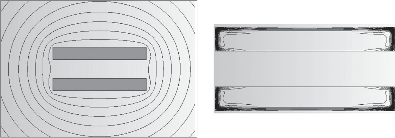
Visualization of electromagnetic field contours showing the 'swirling' nature of fields around conductive structures, as described by the curl operator in Maxwell's equations.
A Primer on Vector Operators
To interpret Maxwell's equations, analysts use vector operators that simplify complex differential operations. While these can be expressed in various coordinate systems, understanding their physical meaning in rectangular coordinates is essential for setting up simulation boundaries and interpreting field results.
- Gradient (∇U or grad U): Represents the rate of change of a scalar field in space. In modeling, this is used to describe temperature gradients or potential variations across the workpiece.
- Divergence (∇·U or div U): Measures the 'outflow' or 'source' of a vector field from a point. For magnetic flux density, the divergence is always zero, reinforcing the 'no-source' loop behavior of magnetic fields.
- Curl (∇×U or curl U): Describes the rotation or 'swirling' of a vector field. In induction heating, the curl of the magnetic field relates to the current density, while the curl of the electric field relates to the time-varying magnetic field, essentially defining the 'interaction' that leads to eddy current generation.
Constitutive Relations and Material Properties
Maxwell's equations alone are "indefinite" until we specify the relations between the field quantities. For linear isotropic media, we use the following constitutive relations:
- $D = \varepsilon_0 \varepsilon_r E$, where $\varepsilon_r$ is relative permittivity.
- $B = \mu_0 \mu_r H$, where $\mu_r$ is relative magnetic permeability.
- $J = \sigma E$ (Ohm's Law), where $\sigma$ is electrical conductivity, related to resistivity ($\rho$) by $\sigma = 1/\rho$.
Assumptions: Hysteresis and Magnetic Saturation
When formulating a mathematical model, analysts often neglect hysteresis losses and magnetic saturation to simplify calculations. This assumption is generally valid for the majority of induction heating applications for steels, such as through-hardening or heating before forging, rolling, and extrusion. In these processes, the heat effect attributed to hysteresis losses typically does not exceed 6%–8% of the total eddy current losses. This is because, for the majority of the heating cycle, the surface temperature of the workpiece is well above the Curie temperature, rendering the material nonmagnetic.
When to Account for Hysteresis Losses
Include hysteresis in low-temperature applications where the material remains magnetic throughout the process: induction tempering, paint curing, stress relieving, heating before galvanizing, and lacquer coating.
Neglecting hysteresis in these scenarios leads to inaccurate prediction of heating rate and final temperature distribution.
Practical Simplifications for Engineers
In most practical induction heating applications involving metallic materials, the frequency of currents is typically less than 10 MHz. At these frequencies, the induced conduction current density (J) is significantly greater than the displacement current density. This allows us to neglect the displacement current term in Ampere's Law, leading to the simplified expression:
$$\nabla \times H = J$$
This simplification is critical as it reduces the computational complexity of the model without sacrificing accuracy for standard industrial IH processes. Furthermore, many engineering projects can be effectively handled using two-dimensional (2-D) assumptions—either Cartesian or axis-symmetric cylindrical systems—which are much less computationally expensive than full 3-D simulations. 3-D consideration is often discouraged by much higher computing costs, the requirement for specific user experience, and the time-consuming challenges of representing complex geometric input and results.
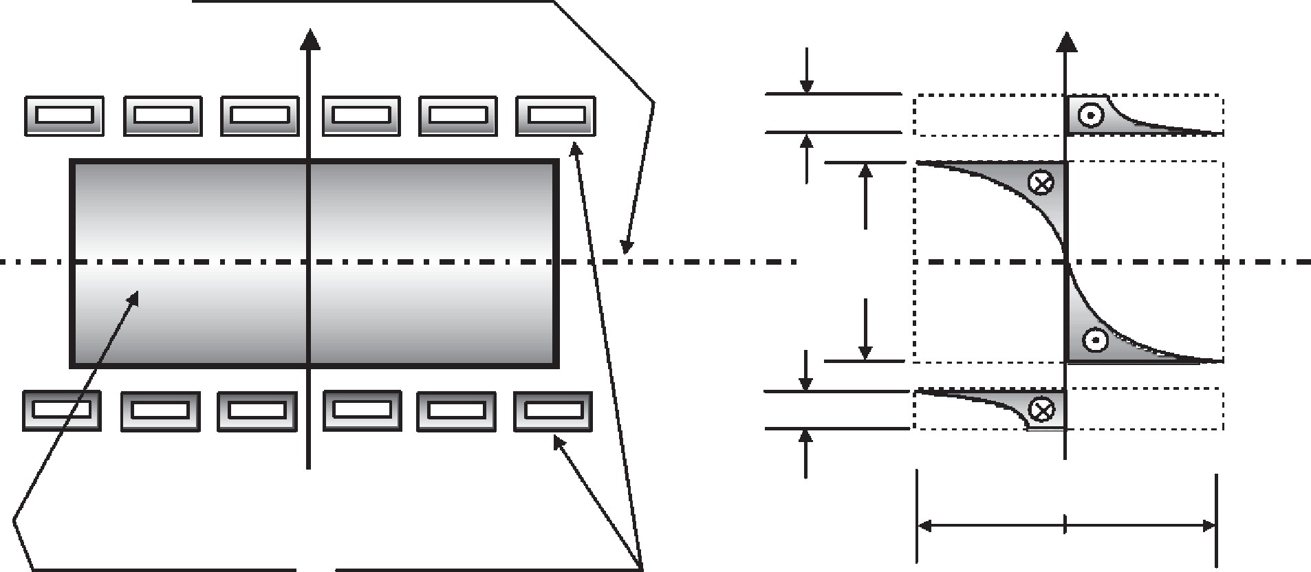
A simplified 2-D axis-symmetric model of a cylindrical workpiece and induction coil, illustrating the distribution of flux density across the radius.
Choosing the Right Numerical Method
Once the governing equations are established, they must be mapped to a numerical method. These fundamental laws can be written in both differential form and integral form (by applying Stokes' theorem). Different numerical methods utilize these different forms, and selecting the right one depends on the application, required accuracy, and time/cost limitations.
| Method | Form | Strengths | Limitations | |
|---|---|---|---|---|
| FEM | Finite Element Method | Differential | Excels at complex geometries and material nonlinearities | Requires full mesh including air regions |
| FDM | Finite Difference Method | Differential | Simple to apply for classical shapes with orthogonal mesh | Less suited for complex boundary configurations |
| BEM | Boundary Element Method | Integral | Mesh only on conductive surfaces; faster execution | Challenges with appreciably nonlinear processes |
| MIM | Mutual Impedance Method | Integral | Fast for cylindrical systems; reduced mesh size | Less accurate for complex-shaped bodies |
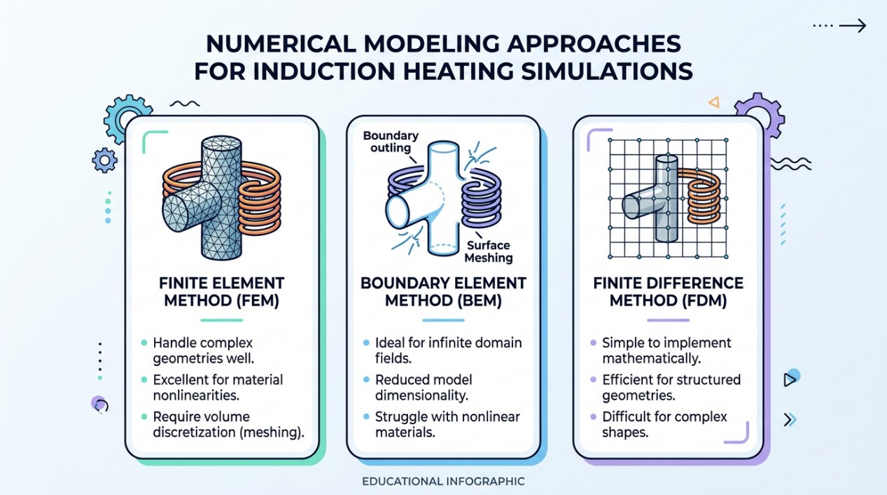
A comparative overview of FEM, BEM, and FDM approaches, highlighting the differences in meshing strategies and application strengths for induction heating.
Model Credibility Checklist
To ensure accuracy and avoid "garbage in/garbage out" scenarios, analysts should follow a rigorous validation mindset based on the following factors:
- Selection of Governing Equations: Verify that the chosen theoretical model properly describes the technological process. For metallic IH < 10 MHz, confirm if frequency-based simplifications (neglecting displacement current) apply.
- Assumption Check: Review assumptions such as steady-state quality (time-harmonic representation) and whether hysteresis/saturation can be safely neglected based on the temperature range (e.g., above vs. below Curie).
- Material Property Sensitivity: Ensure conductivity ($\sigma$) and permeability ($\mu$) are accurately defined as functions of temperature and field intensity. Poorly defined properties are a major source of modeling errors.
- Boundary Conditions: Carefully define Dirichlet (fixed potential) or Neumann (zero gradient) conditions. At surfaces, account for highly nonlinear losses due to convection and thermal radiation.
- Validation Mindset: Always treat numerical results as approximate engineering solutions. Perform sensitivity analysis on poorly defined parameters, such as initial temperature distributions, and compare results with experimental data or analytical solutions when possible.
FAQ about Induction Heating Simulation
Q: Why can't I just rely on physical prototypes instead of simulation for induction heating design?
Physical prototyping is costly, time-consuming, and often impractical for resolving complex thermal profiles. Simulation allows you to predict how nonlinear factors affect heating outcomes, test different coil geometries and frequencies quickly, and avoid expensive surprises during production. It transforms induction heating from trial-and-error into a predictable engineering process.
Q: When should I account for hysteresis losses in my induction heating model?
For most high-temperature applications like through-hardening, forging, or rolling, hysteresis losses are negligible (6–8% of total losses) because the workpiece heats above the Curie temperature and becomes nonmagnetic. However, for low-temperature processes like induction tempering, paint curing, or stress relieving, the material remains magnetic throughout, making hysteresis losses significant and necessary to include for accurate predictions.
Q: Should I use 2-D or 3-D simulation for my induction heating project?
Most engineering projects can be effectively handled with 2-D models (Cartesian or axis-symmetric cylindrical), which are computationally faster and easier to set up. Reserve 3-D simulations for cases where geometry complexity absolutely demands it, as they require significantly more computing resources, specialized expertise, and time for both setup and result interpretation.
Conclusion: Induction Heating Simulation and Maxwell's Equations
By grounding simulation efforts in the fundamental laws of electromagnetism while applying practical engineering simplifications, specialists can transform induction heating design from a trial-and-error "black art" into a precise, predictable science. The goal is not just a "pretty graphic," but a technically adequate result that matches practice and prevents failure.
Keep Learning
Power Supplies by Application Family: Joining, Mass Heating, and Strip Processing
Key Takeaways Joining operations (brazing, soldering, bonding) demand higher frequencies and matching flexibility to handle variable coil coupling and precision surface heating. Mass heating lines (billets, bars, slabs) prioritize continuous duty, efficiency, and ruggedness at high power levels with multi-coil zone control. Strip processing requires architectures that separate control electronics from high-frequency inverter modules to cope with harsh installation environments. Specifying only kW and ......
Simultaneous Dual-Frequency Induction Power: When One Frequency Forces the Wrong Compromise
Key Takeaways Dual-frequency is justified by robustness, not complexity: It should only be adopted when a single frequency forces an unacceptable compromise between surface and bulk heating requirements. Give each frequency a defined role: Assign the lower frequency to bulk heating/penetration and the higher frequency to surface shaping—then develop recipes one variable at a time. The combining network is the engineering center of gravity: Frequency-selective coupling paths, thermal rating for worst-c......
Applying Induction Power Supplies in the Real World: Constraints That Decide Uptime and Quality
Key Takeaways Application constraints dominate real-world performance: Two induction systems with identical kW ratings can behave very differently depending on cable length, cooling water temperature, dust levels, and fixture repeatability. Design for drift, not for perfect day one: Coils deform, filters clog, sensors drift, and connectors loosen under thermal cycling. Baseline monitoring during commissioning is essential. Mechanical repeatability often beats control complexity: Improving fixturing an......
Medium- and High-Frequency Transformers in Induction Systems: Design Drivers Engineers Should Actually Care About
Key Takeaways Not Passive: Transformers set the electrical operating point for the entire induction station—coil voltage, current, capacitor stress, and inverter margin all depend on transformer choice. Frequency Effects: At higher frequencies, winding losses and stray capacitance dominate; a transformer that looks fine on turns ratio can fail a duty-cycle test if loss distribution is wrong. Placement Matters: Moving the transformer and capacitor bank closer to the coil reduces high-frequency loop len......
Load Matching in Induction Heating: Designing for Stability, Efficiency, and Real-World Variation
Key Takeaways Dynamic Load: Induction heating loads are not fixed—coupling, material properties, and temperature all shift impedance during operation, making matching a continuous design challenge. Q Factor Matters: High-Q loads can produce large circulating currents and capacitor stress even at modest delivered kW; design for the worst-case kVA, not just power. Discrete Ranges Win: Transformer taps and capacitor steps that cover discrete matching ranges outperform a single broad-range configuration f......
Induction Power Supply Topologies: A Practical Guide to Converters, Inverters, and Matching Networks
Key Takeaways Point 1: Topology choices determine input power quality, response speed, detuning tolerance, and physical constraints in real installations. Point 2: Converter options (diode vs SCR vs active front end) significantly affect partial-load power factor and plant power quality. Point 3: Inverter types (voltage-fed vs current-fed) dictate protection philosophy and sensitivity to load changes, while matching network placement is driven by cable length limitations. Induction heating power suppl......